The next eshine telescope

Some CCDs are not 2-dimensional, but are just a single line of sensors. Typically used for scanning devices. Here is one such. Another is here.

The first one appears to be 16 bit – but what is the readout noise, and can you get line CCDs with better than 16 bit dynamic range? Second one is an 11ish bit device?

There is a type of camera where the sensor reacts to changes, not to ‘an exposure signal’. The DAVIS 346 Neuromorphic camera is one such.

Data-sheet: https://inivation.com/wp-content/uploads/2019/08/DAVIS346.pdf

Note the apparent high dynamic range of 120dB – like a 100-image stack from MLO?

Wiki: https://en.wikipedia.org/wiki/Event_camera

How can we use an ‘event-based camera’? Can the camera also be triggered from outside?

We have received help with the software that extracts images from the Sigma SD10 X3F files. These are RAW files packaged in a special way. The software is ‘x3f_extract’, provided at proxel.se by Roland Karlsson. The code can be downloaded at http://proxel.se/x3f.html

A small modification of the code is needed to avoid ‘clipping’ of pixel values below the mean of the bias level. The modification must be introduced into the source file and then code must be recompiled. The code to modify is inside the ‘src’ directory that is built when you download all the source files from proxel. Inside the code ‘x3f_io.c’ go to the routine “huffman_decode_row” and find the line:

uint16_t c[3] = {0,0,0}, c_fix[3];

comment it out and exchange it with:

uint16_t c[3] = {100,100,100}, c_fix[3];

Then go one level up and run ‘make’.

I did the above and took some dark frames that I averaged in the half-median-half-mean way, in each pixel. I generated row and column sums of these dark frames and got this:

The structure is low, actually, at the 1 count level.

With this fix of the x3f_extract code we have no longer a ‘strange clipping’ problem and the SD10 can be used for astrophotography – the point being that when its internal IR filter is removed and a red filter i used over the lens we have in effect a camera able to perform VE1 and VE2 band photometry in one shot, without any moving parts. We have yet to do the image manipulations required to reduce the images obtained in the R G and B channels to R G and IR values – but that will happen.

We test Hans’ 450D optics by imaging the Full Moon (t_exp = 0.02 s, f=5.6, focal length=300 mm (i.e. tele-lens)). Using IRIS to extract the R G and B fields we align, normalize and average these and plot the profile from Moon disc centre and out into the halo. We get:

The red, green and blue curves represent the halo in R G and B, respectively. The black line is a 1/r³ curve. R, G and B images normalized by their total flux before plotting.

It would seem that, as in the case of the image found on the internet, the profiles of R G and B are very similar, and also of ‘high quality’ – i.e. they are almost at the limit of what is possible in terms of dropoff slope.

This has bearing on choice of future cameras – CMOS or filtered CCD. I think the similarity of the profiles is due to the light having traversed the same optics – which is not the case with the filter-wheel.

I am not sure why the profiles are so close to 1/r³. It seems our optics in the MLO telescope cannot match this.

It should be said that the DSLR optics show ghosting – this can interfere with the DS photometry if unluckily placed – but apparently does not gives us shallow halo profiles.

The ghost image (same size as Moon, positioned at 11 o’clock) is due to internal reflections in the compact tele-lens used. Perhaps an image of the Moon is reflected from the CMOS surface, reflects off the back of the optics and is recorded. The above ghost would be very intense compared to the DS. Similar ghosts are seen in the wide-angle lens image taken with the Sigma camera, but as magnification is less the ghost is easily placed away from the Moon.

One thing to notice is the 2-orders of magnitude of drop in intensity from the disc brightness to the start of the halo – is this what we get with our MLO telescope? Perhaps the 1/r³ drop is an artifact of a high starting level? Need to check that.

IRIS is a piece of Windows software that will readily convert CR2 files into FITS files. It can be done via pull-down menus or via ‘scripts’

A typical script is:

loadcam IMG_7536
save IMG_7536
loadcam IMG_7537
save IMG_7537
loadcam IMG_7538
save IMG_7538
loadcam IMG_7539
save IMG_7539
loadcam IMG_7540
save IMG_7540
…

Image files named IMG_XXXX.CR2 are here being loaded and saved as 16-bit FITS named IMG_XXXX.fit

It is necessary to first, via pull-down menus, set up IRIS to expect a Canon EOS camera (hence it understands to look for CR2 files in the script). You must also set the paths (in Settings…) to where the data are and where the scripts are. When you want to process .X3F images you must pick the SIGMA SD10 camera from the ‘camera’ menu in IRIS.

The script is a text file with extention ‘.pgm’ and is run from the ‘console’ in IRIS – this is the 11th icon along the toolbar. Simply write

RUN nameofscript (omit the .pgm, apparently)

and it will run, saving files for you.

X3F files are not yet understood – IRIS will open a file and save a FITS but there is only one ‘colour-plane’ in the FITS file – in the CR2 files converted above we get 3.

IRIS can be run from ‘wine’ in Ubuntu.

A quick
search on Internet gives many references to DSLR
photometry. Amateur astronomers use DSLRs to observe stellar light curves
(see the AAVSO web
site) and to search for exoplanet transits, sometimes in the form of
amateur/professional collaborations (PANOPTES). There are also examples of the
use of DSLRs in the scientific literature: Velidovsky et al., used a Canon EOS 300D for absolute
photometry of the Moon.

Since I own
an old Canon EOS 300D I thought I’d try to measure a few fundamental
parameters: readout noise, dark current, and gain factors. The EOS 300D model
is now 10 years old and must be regarded as obsolete. I’ve seen them sold at
Ebay for less than 50 USD. It has a 12-bit 3088×2056 CMOS sensor, ISO settings
from 100 to 1600, exposure times from 0.25 milliseconds to 30 seconds, bulb
exposure of infinite length, but unfortunately no mirror lockup. I used IRIS to
convert files from RAW to FITS (note: without debayering the images), and IDL
for the actual analysis.

The gain
factors were determined by taking pairs of exposures from 0.25 to 100 milliseconds,
selecting a 600×400 pixel sub-frame, and plotting the variance of the
difference frame versus the mean level. Image
sequences were generated for ISO 400 and ISO 800, and the R-, G-, and
B-channels (of the Bayer matrix) were treated as independent data points. The
exposures were taken without lens, and with the camera pointed at a white,
uniformly lit wall. At first, the data points spread out across the graph but
when I discarded all exposures shorter than 10 milliseconds, the remaining data
points fell nicely along a straight line. For shorter exposure times, there is apparently
a large spread in the shutter performance (assuming that the light source is
constant between exposures). The uncertainty fell below 1% for exposure times
longer than around 50 milliseconds. This shutter performance may be a property
of the camera model, but it may also be a consequence of my camera being old
and worn-out.

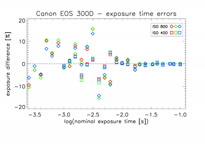
Figure 1. Percentage difference between pairs of exposures at different nominal exposure times.

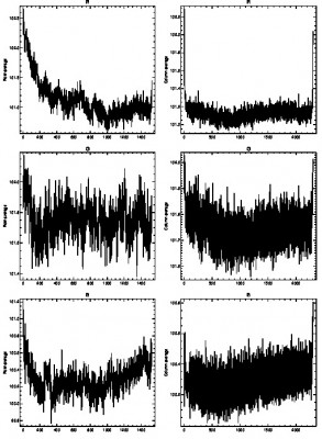
The obtained
gain curves are shown in Figure 2. The resulting gain factors are g=2.58 electrons/ADU at ISO 400 and g=1.17 electrons/ADU at ISO 800,
which comply well with figures that I found at various web sites (here,
here). Above a signal level of around 3700
to 3800, the gain curves rapidly levels off to smaller noise values, indicating
an abrupt transition from linearity.

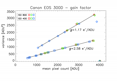
Figure 2. Variance of noise versus signal for ISO 400 and ISO 800.

Readout
noise and dark current was determined by repeating the above experiment, but now
with the camera body capped and going to exposure times longer than 20 minutes.
Figure 3 shows a surprising result: the dark current decreases with time, to levels below the CMOS bias level (128 for
the EOS 300D) which means negative values!
Clearly unphysical, but it could be explained as a consequence of
onboard dark-current subtraction before the CMOS frame hits the RAW file.
Apparently, the camera over-estimates the dark current. Or could it be IRIS
that does these subtractions in the RAW-to-FITS conversion?

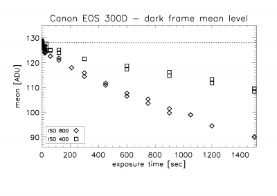
Figure 3. Dark current as a function of exposure time.
This behavior can only be
explained by onboard dark current subtraction before storage in the RAW file.

Even if the
dark current signal have been
subtracted in the RAW frame, the dark current noise is still there and this may tell us something about the dark
current signal. Figure 4 shows the dark
current variance as a function of exposure time. Up to 7 or 8 minutes it is a
roughly linear relation, but then the curve bends upwards – more strongly for
the ISO 800 sequence. The camera warms up during long exposures (one can
actually feel the temperature difference) and this is a likely explanation for
the nonlinear behavior in Figure 4. This is actually one of the major
limitations of DSLR cameras: the lack of temperature control causes a time
dependent behavior of the dark current, which is difficult to predict or to
monitor.

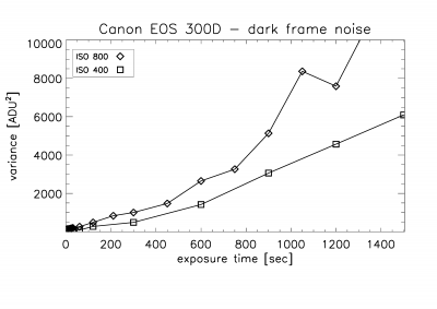
Figure 4. Dark current noise (here, the variance) as a
function of exposure time.

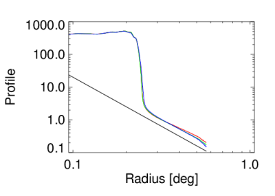
The readout noise can simply be obtained as the dark current for zero exposure
time. In Figure 5, we expand Figure 4 by plotting the logarithm of the observed
noise (but now the standard deviation) as a function of the logarithm of the
exposure time. Assuming that the observed noise is a combination of readout
noise and dark noise, and that the dark noise is proportional to the square
root of the exposure time (which it should be for exposures shorter than 5 to
10 minutes), we can fit both the readout noise and the dark current to the
observed data. Using the gain factors obtained above, we get a readout noise of
13.7 or 12.2 electrons, for ISO 400 and ISO 800, respectively, and a dark
current of about 3.6 electrons/pixel/second. This latter figure is highly uncertain,
but it suggests that for exposure times shorter than about 30 seconds the
readout noise dominates.

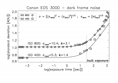
Figure 5. Dark current noise (here, the standard
deviation) versus exposure time on logarithmic scales.

Some
conclusions:

–
Gain
factors and readout noise obtained are relatively consistent with those found
by others. The dark current is a bit on the high side, but cannot be determined
very precisely.

–
The
camera shutter does not allow exposures shorter than 50 msec with any precision.

–
The
lack of temperature control makes the dark current unpredictable. This is less
of a problem for exposures shorter than 30-60 seconds, since they are dominated
by readout noise.

–
There
is some processing going on before the RAW file, at least a dark current
subtraction.

Even the least processed images – those in RAW formats – do not consist of the
raw, unprocessed data in the way we are used to from astronomical CCD cameras.
The details of this onboard processing are not described by the camera manufacturers. A
simple subtraction of a mean dark current level should not pose a problem for
the ability do photometry. However, if the processing includes scaling,
filtering, bad-pixel removal, “noise reduction”, etc., it may introduce
unpredictable errors in photometric measurements. How can we test this?

In this entry we found some puzzling results. Ignore them! The variance had been screwed up by incorrect procedures on my part. As Hans pointed out, you have to use the method where two images with same exposure (and they must be of an evenly lit surface) are subtracted – the difference has twice the variance of each of the images. This method cancels various common features in the images – blemishes in the flat target as well as uneven response in the chip, and dust on the chip.

Taking a series of twin exposures from very dark to very bright of a white sheet of paper, and extracting a nice square from this, calculating its mean and variance as per above, we get the following result:

In each panel statistics for R G or B are shown. The readout noise RN is basically the intercept. The Gain is 1./(the slope) of the regression. Two sets of images had to be taken and it would seem the illumination was not even, hence the scatter. Nonlinearities set in for R G and B at various levels – the extent of the x-axis shows the data that are not obviously past the linearity point. So, despite the camera being advertised as 12-bit it has almost 13 bits. Sticking to the 12 seems a good idea – it is all that B can handle, for instance.

We used x3f_extract from proxel.se to extract the R G and B fields from the compressed format X3F files.

This paper by Hytti gets nearly the same as we have above – at least for the G band:

The X3F format images thatthe SIGMA SD10 camera produces are some form of compressed RAW format. It can be dumped out as decoded TIFF files using the

x3f_extract software from the toolkit available at

http://www.proxel.se/x3f.html

I have taken a set of test images of a test card with the internal IR filter removed from the camera, and a Wratten 25A red filter on the lens (and a standard UV-blocking filter). I exposed from a normal setting and with longer and longer exposure times until the images were evidently saturated in all colours, judging from the little histogram on the back of the camera.

After conversion to 16-bit TIFF and reformatting to FITS the mages were inspected and the histograms plotted. As exposure times increased the high edge of the histogram wandered up until it hit some sort of barrier near 10000 counts. This must be the actual saturation level of the camera. It is advertised as 12-bit but that would imply a ḿaximum count near 4096. So it seems we have maybe one bit more than 12 -> 13.

This is a plot of mean value vs standard deviation of a selected square on the test card. There is a linear relationship between S.D: and the mean value … I thought it was mean value and variance … but it breaks down at high mean values.

Added later: Ignore the plot. Look here instead: link